

Study design
A subset of participants with genetic data from the USDA Nutritional Phenotyping Study (ClinicalTrials.gov: NCT02367287), a cross-sectional study conducted at the USDA Western Human Nutrition Research Center (WHNRC) in Davis, CA, were included in this analysis (n = 211). A detailed description of participation and study design for the Nutritional Phenotyping Study has been previously published [9]. Briefly, generally healthy adults between the ages of 18–66 years were recruited and enrolled. Sex was used as a binary categorization and participants self-reported as either female or male during the initial screening process. Participants were excluded if they were pregnant, lactating, had undergone minor surgery recently or major surgery in the past 16 weeks, were hospitalized 4 weeks prior to their scheduled study visit, or were taking antibiotic therapy or daily medication for a diagnosed chronic disease.
Following initial screening and enrollment into the study, participants attended 2 study visits ~2 weeks apart. During the first study visit, a self-reported demographic questionnaire was given to participants and physiology measures, including body composition and fitness, were taken. On the second study visit, resting metabolic rate (RMR) and blood samples were collected following a 12-h overnight fast and after the consumption of a standardized mixed macronutrient meal challenge.
Ethics approval and consent to participate
All methods were performed in accordance with the relevant guidelines and regulations. The study was approved by the University of California, Davis Institutional Review Board (protocol: #691654). Participants provided written informed consent and received monetary compensation for participation in this study.
Body composition
Body weight and height were measured using a calibrated scale and wall-mounted stadiometer, respectively. Body fat and lean mass were measured using dual x-ray absorptiometry (DXA, Hologic Discovery QDR Series with Apex 13.3.7, Hologic, MA, USA) by a trained and licensed technician. Pre-menopausal female participants reported the date of their last menstrual period and completed a spot urine pregnancy test prior to scan. Whole body scans were performed on participants to provide data on total lean body mass and total fat mass. Body fat percentage (BF%) was an output from the DXA scan, reflecting the total fat mass divided by the total body mass. Lean mass index (LMI) was calculated as total lean body mass (kg) divided by squared height (m2). The “trunk” is the area starting from the bottom of the chin to the pelvis, excluding the arms and legs. Trunk fat percentage (TF%) was an output from the DXA scan. The trunk area consists of the android and the gynoid region. Android fat mass is fat accumulation in the area 20% of the distance from the crest to the chin, excluding the extremities, while gynoid fat mass is fat accumulation in the area around the hips/pelvis. The android-to-gynoid fat mass ratio (AGR) was used to infer the distribution of fat mass and calculated as the total android fat mass divided by the total gynoid fat mass. In the manuscript, we use the term adiposity to refer to body fat measured by DXA, including regional fat distribution.
Metabolic syndrome traits
The five classical Metsyn traits – waist circumference, fasting triglycerides (TG), fasting high density lipoprotein cholesterol (HDL-c), fasting glucose, and blood pressure (systolic (sBP) and diastolic (dBP)) – were collected in the study. Waist circumference was measured at the smallest horizontal circumference between the ribs and iliac crest. Fasting plasma TG, HDL-c, and glucose were measured on a Cobas Integra 400 Plus (Roche Diagnostics Corporation). Seated blood pressure measurements were obtained using the CARESCAPE V100 Vital Signs Monitor (GE Healthcare) following a 5 to 10-minute rest.
Dietary assessment
Dietary recalls were obtained using the Automated Self-Administered 24-hour (ASA24) dietary recall tool from the National Cancer Institute of the National Institutes of Health [10]. A detailed description of the dietary data collection and processing has been previously published [11]. Briefly, participants were familiarized with the ASA24 dietary recall process by trained personnel and were guided on how to report food intake online. In the 10–14 days between study visits, participants were prompted to complete 3 unscheduled recalls at home, which were split between 2 weekdays and 1 weekend day to account for variations in food intake throughout the week. Dietary quality for 3-day food intake averages was assessed using the Health Eating Index (HEI), which estimates adherence to the US Dietary Guidelines for Americans [12]. The total HEI score was used for estimating dietary quality in analyses.
Resting metabolic rate (RMR)
Prior to the second study visit, participants consumed a standardized dinner meal and ceased any food or beverage consumption (except for water) 12 h before their scheduled visit to the center. Upon arrival, a trained physiologist measured RMR through indirect calorimetry by a metabolic cart (TrueOne 2400, ParvoMedics, Sandy, UT). Participants laid semi-reclined and were undisturbed for 5 min prior to testing. Respiratory gases were then collected for ~15–20 min to measure oxygen consumption and carbon dioxide production. These data were used in the Weir equation (without urinary nitrogen) to estimate RMR [13]. RMR was subsequently divided by body mass to account for innate differences in RMR due to body size.
Fitness
The YMCA 3-minute step test is a validated exercise test to evaluate participant cardiorespiratory fitness [14, 15]. Prior to the fitness assessment, the Physical Activity Readiness Questionnaire (PAR-Q, American College of Sports Medicine, Indianapolis, IN) was administered to determine if the participant could complete the exercise test safely [16]. Participants who answered “yes” to any of the questions in the readiness questionnaire related to heart, bone, or joint conditions, or recent injuries were categorized as “Unknown” for fitness level. For the fitness assessment, a heart rate monitor (Polar Watch V800, Polar Electro, Kemplele, Finland) was secured to the wrist and resting heart rate was collected. Participants stepped up on a 12-inch box, one foot at a time, and then stepped down, one foot at a time, for 3 min. A metronome set to 96 beats per minute was used to indicate when participants should step with the alternating foot. Seated heart rate was measured during the first minute of the recovery period. The post-exercise heart rate was stratified using participant age and sex to categorize them into “Very Poor,” “Poor,” “Below Average,” “Average,” “Above Average,” “Good,” or “Excellent” fitness levels.
Genotype data
Participants consented to genotyping and samples were prepared using PAXgene Blood DNA kits (Qiagen, Germantown, MD) for sequencing, which has been described previously [17, 18]. DNA was extracted and purified according to the manufacturer’s instructions and sent to UCLA Neuroscience Genomics Core for genotyping. The Infinium Global Screening Array version 3 (Illumina Infinium GSA-24 v3.0 BeadChip) was used to type 654,027 high-quality SNPs across the human genome. Data underwent quality control measures including excluding duplicate single nucleotide polymorphisms (SNPs), low quality (<95%) genotyping and missing SNPs (>1%), SNPs that fail Hardy-Weinberg Equilibrium (HWE < 0.0001), monomorphic SNPs, SNPs with an indeterminate allele, and SNPs that map to multiple probes. Related participants with an identity by state value greater than 0.2 were identified, and inclusion of relatives was evaluated for impact on downstream analysis. Genetic data from the sample was subsequently imputed using the TOPMed imputation server to impute the genotype array data. The server facilitates a multi-step process to enhance genotype accuracy including quality control to filter out low-confidence genotypes. Briefly, the genetic data, originally in Hg19, underwent LiftOver followed by quality control, which returned a reference overlap of 93.79% (chr 1–10), 93.99% (chr 11–22), and 92% (chr X) with the TOPMed R3 Hg38 reference panel. Principal component (PC) analysis was used to generate PCs which account for overall genomic variation and population structure. The first 5 PCs were utilized in analyses and describe >50% of the genetic population structure.
PRS calculation
Polygenic risk scores describe the combined risk of several risk-inducing SNPs previously identified in GWAS. The PRS for BMI was calculated using the PGS Catalog and pgs_calc pipeline [19] made accessible by the nf-core community [20]. Briefly, the harmonized GRCh38 PGS002313 score file, from Weissbrod et al, was downloaded from PGS Catalog and subsequently used in pgs_calc along with the study sample’s imputed genetic data [21]. This score was based on the cumulative effect of more than 1 million genetic variants identified through large-scale GWAS in the UK Biobank. The pgs_calc pipeline matches variants in the scoring files against variants in the target dataset and calculates PRS for all samples (using linear sum of weights and dosages). The target dataset (USDA Nutritional Phenotyping Cohort) was an independent sample from the discovery GWAS (UK Biobank). Genetic variant coverage was high for this PRS (96.1%). The calculated PRS was then normalized and centered around 0 prior to inclusion in the analysis models (Supplementary Fig. 1). PRS quintiles were utilized only in data visualization to compare the BMI between low, medium, and high-risk groups as the genetic effects were more likely to manifest in the extremes; PRS quintile 1 was assigned “low-risk”, PRS quintile 2, 3, and 4 were assigned “mid-risk”, and PRS quintile 5 was assigned “high-risk.” The continuous, normalized PRS variable was utilized in the subsequent linear regression models.
The PRS was validated using a larger sample set of the USDA cohort (n = 230) of participants with age, sex, BMI, and genetic data. BMI was used to classify participants with obesity (BMI > 30) and subsequently used to find the discriminate ability of PRS to identify participants with obesity using area under the receiver operating curve (AUROC). A linear regression model was used to evaluate the association and R2 of PRS predicting BMI after adjusting for age, sex, and principal components.
Independent associations with DXA phenotypes
Spearman correlations were used to assess monotonic relationships between selected variables and covariates (Fig. 1). The critical Spearman’s rho value for statistical significance was approximated based on a sample size of 211 and a significance level of 0.05.
Fig. 1: Spearman correlation plot.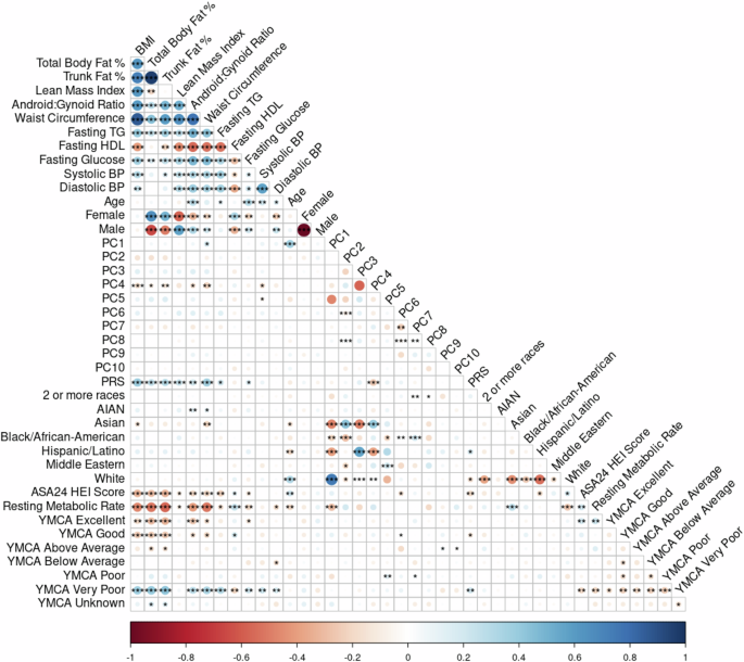
The plot of the Spearman correlations including all predictor and response variables examined in this sample (n = 211). Associations between variables are colored according to the sliding gradient from red (−1) to blue (1) and significant associations are denoted by asterisk (*<0.5, **<0.01, ***<0.001). Among the covariates, fitness shows a moderate correlation with the DXA phenotypes, as does HEI, indicating some association between fitness level and dietary quality with body composition. PRS is correlated with DXA phenotypes, supporting the role of genetic factors in body composition variation. Notably, the first 5 principal components (PCs 1–5) describing the genomic variation and population structure (cumulative eigenvalue = 20.8) show distinct correlations with the reported DXA phenotypes, age, PRS, and other variables, while PCs 6–10 are largely redundant (PC 1–10 cumulative eigenvalue = 28.5). This redundancy suggests that only the first five PCs are of primary interest in subsequent analyses, as they capture the most meaningful variation across the phenotypes. Additionally, these PCs exhibit significant correlations with the participant’s self-reported race.
Linear regression models including all standardized predictor variables were used to assess percent variation using sum of squares to describe the independent contribution of each predictor to each outcome. Variance inflation factor was used to assess multicollinearity.
Full model building
PRS, HEI, RMR, and fitness variables were evaluated along with age, sex, and genetic PC 1–5 in a full model. First, variables were standardized, mean centered with an SD of 1, to ensure comparability in combined models by making each variable more consistent and easier to understand. Next, variables were examined using sum of squares and partial R2. The sum of square criteria measures the contribution of each predictor, without accounting for the influence of other variables, while the partial R2 criteria measures the unique contribution of each predictor accounting for the remaining variables. Models for each phenotype were subsequently evaluated using stepwise, bi-directional regression analysis and evaluated using Bayesian information criteria (BIC) to determine the most explanatory model. Each regression model was iteratively built by adding and removing variables, alternating between forward and backward selection at each step, using BIC to determine which variables to keep in the model at each iteration using the MASS package in R [22].
Statistical methods and computing
R (Version 4.4.1, R Foundation for Statistical Computing; Vienna, Austria) [23] was used for statistical analysis and visualizations. Distribution transformations for PRS were described above. DXA phenotypes and covariates were normalized, if necessary, using logarithmic transformations; BMI, LMI, waist circumference, fasting TG, and fasting HDL-c were normalized, distribution histograms are in Supplementary Fig. 2. A significance level of α = 0.05 was used throughout the manuscript. This research was supported by the Ceres High-Performance Cluster computing network hosted by USDA-ARS.


