

Protein preparation and structural optimisation
In the initial structural analysis of the considered DNA gyrase protein from P. aeruginosa, residues at positions 102–119 were found to be missing. To address the issue of DNA gyrase and to repair any missing atoms in the Colicin E9 immunity protein, both proteins were selected for homology modelling using the SWISS-MODEL tool44, utilising the same template structure as the original PDB entry. To check the closeness of the prediction, the crystal and modelled structures of DNA gyrase and Colicin E9 immunity protein were superimposed, as shown in Fig. 1. Both structures were closely aligned, with only slight deviations. From the superimposed structures, the RMSD was calculated to quantify structural similarity. The RMSD values were found to be 0.491 Å for DNA gyrase and 0.447 Å for the Colicin E9 immunity protein, respectively. The low RMSD values for both proteins indicate similar predictions with high accuracy. The local loop region of the broken part and modelled portion was superimposed (Fig. S1 in the Supplementary file), and RMSD was calculated. Low RMSD of 0.836 Å indicated the close prediction of the broken portion of the DNA gyrase protein. Furthermore, structural validation of the modelled DNA gyrase protein and Colicin E9 immunity protein was conducted to assess their quality and suitability for subsequent computational analyses, including the SAVES server and 50 ns of MD simulation.
Fig. 1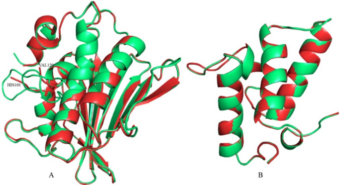
Illustrating the structural comparison between the crystal and modelled proteins. Red and green colours represent the crystal and modelled structure, respectively. (A) DNA gyrase, and (B) Colicin E9 immunity protein. Amino acids at the broken part of the DNA gyrase are labelled.
Validation using the SAVES server
The original crystal structures, along with the final frames of the 50 ns MD simulation trajectories for both proteins, were used to derive several statistical parameters from the SAVES server30, which are given in Table 1. Particularly, the Errat score, which evaluates the quality of non-bonded atomic interactions, indicated excellent structural integrity for both proteins. The modelled DNA gyrase structure had an ERRAT score of 94.3, which declined slightly to 92.0 after 50 ns of MD simulation, indicating minor structural adjustments during optimisation. In a similar manner, the Colicin E9 immunity protein started with an Errat score of 97.3, decreasing to 89.2 following simulation. The evaluation of the Ramachandran plot confirmed the stereochemical integrity of both models. For DNA gyrase, the crystal structure showed that 88.6% of residues were located in the most favourable regions. This figure increased to 89.8% after the MD simulation. At the same time, the proportion of residues in the additionally allowed areas decreased from 11.4% to 8.5%, while no residues were located in disallowed regions, signifying improved stereochemical stability. Regarding the Colicin E9 immunity protein, the most favourable regions increased from 91.8% to 94.5%, and residues within the additionally allowed areas diminished from 8.2% to 5.5% post-simulation. Also, for DNA gyrase, no residues were detected in the disallowed regions of the Colicin E9 immunity protein, indicating high-quality structural modelling.
Table 1 Statistical metrics from the SAVES server for DNA gyrase and Colicin E9 immunity protein before and after 50 ns MD simulations.Validation through molecular dynamics simulation
A 50 ns MD simulation was conducted on the reconstructed DNA gyrase and Colicin E9 immunity proteins, using homology modelling to refine their structures and assess stability. These simulations were performed in a solvated environment with ionic conditions that reflect physiological states. The structural deviations were assessed by calculating backbone RMSD values for both proteins before and after the 50 ns MD simulations. The structural integrity of both DNA gyrase and Colicin E9 immunity protein was found throughout the simulations (Fig. 2A). No individual frame showed deviations greater than 0.3 nm. Furthermore, the patterns of amino acid fluctuations noted during the dynamic states displayed no irregularities (Fig. 2B). The rigidity and compactness of both proteins remained intact throughout the MD simulation (Fig. 2C). The changes in SASA for both proteins during the dynamic states indicated proper protein folding (Fig. 2D). The data from the MD simulations of both proteins reflected their stability and rigidity, as well as their robustness in dynamic states. Thus, the coordinates from the MD simulation were free of close contacts or overlaps, making them suitable for any in silico study.
Fig. 2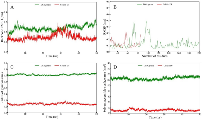
Statistical parameters from MD simulation of DNA gyrase (Green) and Colicin E9 immunity protein (Red). (A) Protein backbone RMSD, (B) RMSF, (C) Radius of gyration, and (D) Solvent accessible surface area.
To comprehend the positional displacement of DNA gyrase and Colicin E9 immunity protein, the final frame from the 50 ns MD simulation trajectories was superimposed onto the homology model structures, and the RMSD was calculated (Fig. 3). The RMSD upon superimposition was found to be 0.891 Å for DNA gyrase and 0.742 Å for Colicin E9 immunity protein, respectively. Although these values reflect minor positional displacements, they have significantly affected the structure’s quality, as assessed by the Ramachandran plot and other parameters in the preceding section.
Fig. 3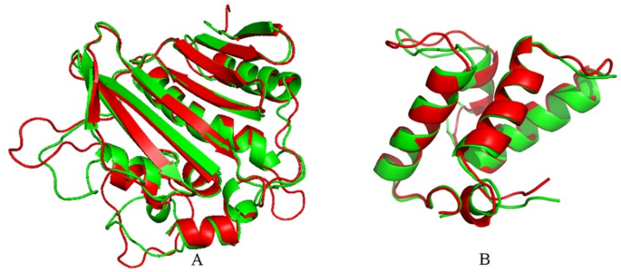
Illustrating the structural comparison between the modelled protein and the last frame from the MD simulation. Red and green colours denote the modelled and MD-simulated structures, respectively. (A) DNA gyrase, and (B) Colicin E9 immunity protein.
Active residue identification
Active-site residues in the DNA gyrase protein were identified using the ScanNet server36, a computational tool that predicts functionally important residues by analyzing structural and sequence features. Figure 4 presents the ScanNet output, highlighting the predicted active site areas, with colours indicating binding probabilities. Specifically, areas marked in blue indicate a binding probability below 0.5, suggesting a reduced likelihood of functional interaction, whereas regions coloured in red reflect residues with a binding probability exceeding 0.5, indicating a higher likelihood of binding. Using the criteria established for the ScanNet server, a comprehensive list of amino acids essential for effective binding interactions with incoming molecular entities was generated. The identified residues include ALA20, LYS23, ARG24, PRO25, GLY26, MET27, TYR28, GLY30, ASP31, THR32, ASP33, ASP34, ASP47, ILE50, ASP51, LEU54, ALA55, TYR57, ARG78, PRO81, GLY104, PHE106, ASP108, ASN109, THR110, TYR111, LYS112, VAL113, SER114, GLY115, GLY116, LEU117, HIS118, ILE187, LYS190, ARG191, ARG193, GLU194, LEU195, PHE197, LEU198, ASN199, SER200, TYR219, GLU220, and GLY221. The spatial distribution of these residues has been meticulously mapped onto the DNA gyrase protein structure, suggesting their role in forming the binding pocket critical for the protein’s catalytic activity and substrate interactions. The active site residues are distributed across diverse regions of the protein, including surface-exposed loops and conserved structural elements, consistent with recognized functional motifs. Future docking research on the Colicin E9 immunity protein will build upon this strategic arrangement, emphasizing the significance of these residues in regulating the protein’s functional profile. These findings not only enhance the understanding of DNA gyrase’s enzymatic function but also provide essential information for the informed development of inhibitors that specifically target this important bacterial enzyme.
Fig. 4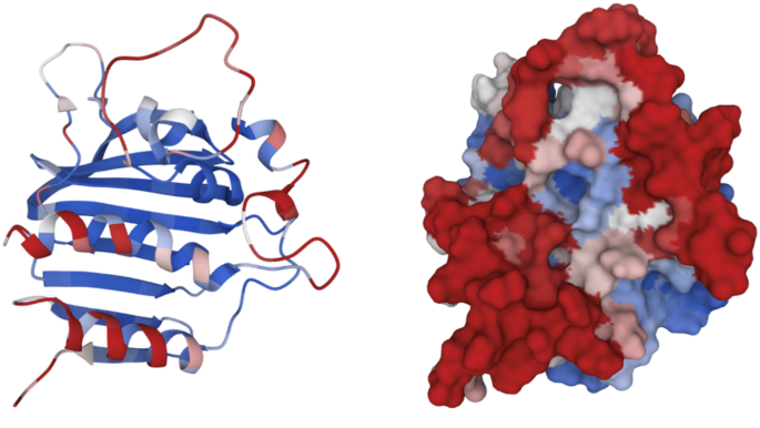
The modelled protein (left) and predicted active site of DNA gyrase (right) of P. aeruginosa were constructed through the ScanNet program based on a geometric deep learning model.
Protein-protein docking analyses obtained through ClusPro and LightDock
Protein-protein docking was conducted to elucidate the interaction between DNA gyrase and the Colicin E9 immunity protein. This investigation employed two complementary tools, ClusPro 2.041 and LightDock42, each utilising distinct docking algorithms to improve prediction reliability. For both tools, the top three docking models were chosen based on their scoring metrics and interaction energies. The leading models from each tool are illustrated in Fig. 5. ClusPro 2.0 generated multiple docking configurations via a clustering algorithm and evaluated them using multiple energy terms, including electrostatic interactions, hydrophobic effects, and van der Waals forces. Models #1, #2, and #3 (Fig. 5A) were selected for their cluster sizes and energy scores. We identified the crucial residues involved in the interaction, which align with the active-site residues suggested by the ScanNet server. Concurrently, LightDock generated docking models (Models #4, #5, and #6 shown in Fig. 5B) by assessing the proteins’ conformational flexibility during their interaction. The top three models were ranked based on their docking energy scores.
Fig. 5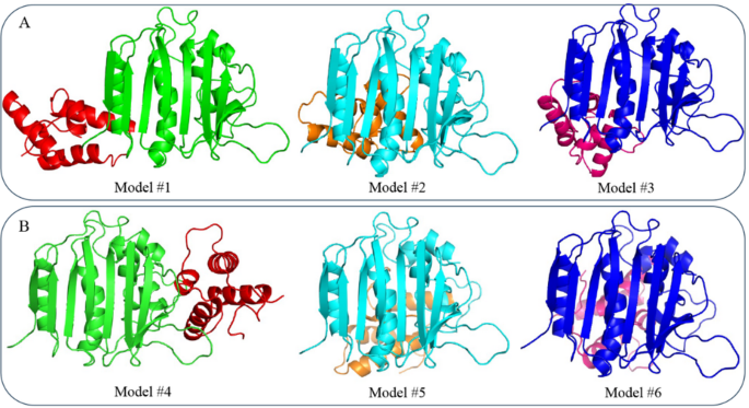
Structural representation of the top three docking models from (A) ClusPro (Models #1 to #3) and (B) LightDock (Models #4 to #6), portraying the interaction between DNA Gyrase and Colicin E9 immunity protein.
Table 2 presents the comprehensive docking results for each model, including components from both ClusPro and LightDock. In particular, the ClusPro weighted score, by means of total interaction energy (E) is represented as a linear combination of different energy terms and expressed by the following expression.
$$E\,=\,{w_{1}}{E_{rep}}+{w_2}{E_{attr}}+{w_3}{E_{elec}}+{w_4}{E_{DARS}}$$
(1)
Each term in this equation represents a specific biophysical interaction at the protein-protein interface, and their relevance is modulated by the weighting coefficients ωn. The weighting coefficients vary depending on the docking mode selected (e.g., Balanced, Electrostatic-favoured, Hydrophobic-favoured). The terms Erep and Eattr represent the repulsive and attractive components of the van der Waals potential, respectively, while setting their coefficients (ω1 and ω2) to values less than 1.0, typically 0.40 in the balanced mode37. The Eelec term represents the electrostatic energy, calculated using a truncated and smoothed Coulombic expression. ClusPro’s balanced scoring scheme uses a significantly higher weight for ω3, specifically 600. The EDARS term represents the pairwise structure-based potential constructed using the Decoys as the Reference State (DARS) approach. DARS is essentially a desolvation potential that models the free energy change associated with the removal of water molecules from the interface upon binding. The DARS term is already scaled to the magnitude of protein-binding free energies, making ω4 = 1.0 the neutral, default weight37.
The results obtained with ClusPro are arranged into clusters, ranked by the number of members that represent docking poses specific to each cluster. In ClusPro, the most reliable prediction is usually the one with the largest member count. Cluster 1 has the highest number of Members (361), significantly more than Cluster 2 (126 Members), with a weighted score of -344.43 for the centre and − 467.88 for the lowest-energy representative, making it the most populated and energetically favourable cluster. It can also be observed that while Cluster 2 has a slightly “better” (lower) Center score (-364.05) than Cluster 1 (-344.43), Cluster 1 is still ranked as Model 1 because its population size is three times larger. In ClusPro, a large cluster indicates a broad, stable energy well, suggesting this docking orientation is the most likely to represent the native state.
Another docking program, LightDock, organizes docking results into swarms and glowworms, representing distinct clustering mechanisms employed in its flexible docking strategy. In LightDock, the score is represented as Luciferin, which is borrowed from the Glowworm Swarm Optimization (GSO) algorithm45. Luciferin encodes the fitness (energetic favourability) of a docking pose. A higher Luciferin value generally indicates a better, more energetically favourable docking pose. The algorithm drives Glowworms (representing potential poses) toward neighbours with higher luciferin levels. The amount of luciferin (l) for a specific Glowworm (i) at a given time step (t + 1) is calculated using the following expression.
$${l_i}\left( {t+1} \right)=\left( {1 – \rho } \right).{l_i}\left( t \right)+~\gamma .~S\left( {{x_i}\left( {t+1} \right)} \right)$$
(2)
Where, ‘\(l_{i} \left( t \right)\)’ is the previous value of luciferin, ‘\(\rho\)’ is the decay constant (default: 0.4), which simulates the “fading” of light over time, ‘\(\gamma\)’ is the enhancement constant (default: 0.6), which determines how much the new energy evaluation affects the score45. Usually, LightDock divides the area around the receptor into hundreds of independent search regions called ‘Swarms’. In the present docking finding, Swarm values (125, 159, and 31) identify the specific geographic starting point on the receptor at which the winning model was discovered. The Glowworm values, found to be 186, 169, and 132, identify the specific point within the swarm that converged on the optimal pose. The Scoring value (top as 23.765) is the numerical representation of the pose’s fitness. Higher values typically indicate more favourable interactions in the LightDock framework. So, overall, each swarm is evaluated based on its score, which indicates the strength and quality of interactions within the predicted complexes. Swarm 1 leads with the highest score of 23.765, making it the top model, followed closely by Swarm 2 at 23.685 and Swarm 3 at 23.423. The quantity of glowworms indicates the sampling density for each swarm, with Swarm 1 having 186 glowworms, the highest amongst all swarms.
Table 2 Summary of docking results for ClusPro and LightDock models.Binding energy and stabilising energy calculation
After successfully completing the molecular docking, the binding energies of the top three models from both ClusPro 2.0 and LightDock were analysed. Further, Gibbs free energy change (ΔG) in protein-protein complexes was estimated using the PRODIGY tool. PRODIGY uses structural properties, including the number and type of interfacial contacts, to predict binding affinities. The predicted and experimentally measured binding affinities demonstrated a Pearson correlation coefficient of 0.73. This approach is advantageous because it can accommodate diverse protein complexes while maintaining consistency across both rigid and flexible binding contexts. The computed ΔG values serve as quantitative indicators of binding affinity between protein pairs, suggesting stronger and more stable interactions. The ΔG for all six models is given in Table 3. All models showed high negative ΔG values, indicating a strong association between DNA gyrase and the Colicin E9 immunity protein. Significantly, Model #2 exhibited the highest binding affinity, with a ΔG of -10.80 kcal/mol, closely followed by Model #6, which had a ΔG value of -10.60 kcal/mol.
Table 3 Binding energy predictions on ClusPro and LightDock complexes.
The stabilising energy for each of the six selected models was calculated using the PPCheck tool, with the results presented in Table 4. It is crucial to note that the stabilising energy serves as a fundamental parameter that provides significant insights into the thermodynamic stability of the complexes by assessing the roles of hydrophobic interactions, hydrogen bonds, salt bridges, and van der Waals forces. Among the various models evaluated, Model #6 demonstrated the highest affinity, achieving a stabilising energy of -65.23 kcal/mol, thereby emphasising its classification as the most stable and energetically advantageous configuration. Among the models produced by the ClusPro tool, Model #2 was recognised as the most stable, exhibiting a stabilising energy of -52.82 kcal/mol. Understanding the stability dynamics among complexes is imperative for identifying the most suitable complexes for subsequent MD simulations.
Table 4 Stabilising energy predictions for the top three docking models from ClusPro 2.0 and LightDock.Selection of best complexes
The binding positions and interaction patterns of all models were evaluated and compared with the active-site amino acids identified by ScanNet through exploration. It was found that Models #1, #3, #4, and #5 from ClusPro and LightDock either failed to reach the active-site residues or were only partially close to them. Since the above models were unable to interact with the hotspot amino acid residues of DNA gyrase, these models were not considered for further analyses. Moreover, analyses of binding and stabilising energies clearly showed that Models #2 and #6 exhibited the highest affinity and stability between DNA gyrase and the Colicin E9 immunity protein. Thus, although Model #2 (from ClusPro) and Model #6 (from LightDock) produced slightly lower scores in docking analyses, they were still regarded as the best models for binding and stabilising energies, warranting further analysis. The overall interaction pattern in three-dimensional (3D) mode was explored and is shown in Fig. 6, indicating that Model #6 exhibited a larger interaction surface than Model #2, which displayed a more compact, focused interface. As shown in Fig. 6, the structural analysis of both complexes reveals key residues and interaction mechanisms that stabilise the protein-protein binding. A significant number of amino acid residues from both DNA gyrase and the Colicin E9 immunity protein were actively involved in the binding interactions, reinforcing the strong association between these two entities.
Fig. 6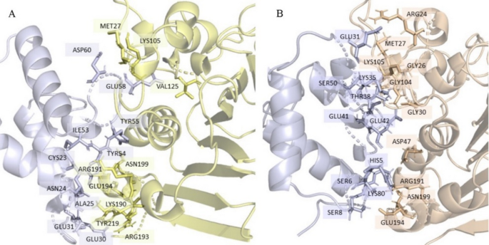
Interaction interface visualisation of (A) Model #2, and (B) Model #6.
Protein-protein binding interaction analysis
The investigation of protein-protein interactions aimed to elucidate the critical residues and forces governing the binding interface of the docked complexes. In accordance with assessments of both stabilising energy and binding energy, Models #2 and #6 were designated as appropriate candidates for subsequent MD simulations, given their demonstrated superior stability and heightened binding affinity. To further clarify the interaction interface, the PDBsum tool was utilized to analyse the docked complexes, as illustrated in Fig. 7. The interaction interface of Model #2 was assessed to identify the essential residues and forces that stabilize the interaction. As shown in Fig. 6, the interface is marked by a multifaceted arrangement of hydrogen bonds, salt bridges, disulfide bonds, and non-covalent interactions, all of which are pivotal in reinforcing the overall stability and specificity of the molecular complex. Table 5 describes a meticulously assembled inventory of amino acids derived from both DNA gyrase and the Colicin E9 immunity protein that are critical to the binding interactions characterised in Models #2 and #6. A comprehensive list of binding-interacting amino acids is given in Table S1 (Supplementary file). It is evident that a broad range of amino acids from both DNA gyrase and the Colicin E9 immunity protein are involved in interactions facilitated by hydrogen bonds, ionic interactions, and hydrophobic forces. The results shown in Table 5; Fig. 7 underscore a significant association between DNA gyrase and the Colicin E9 immunity protein, suggesting that this association plays a vital role in the antibacterial efficacy of Colicin E9. These findings highlight that the interplay between the Colicin E9 immunity protein and DNA gyrase not only impedes bacterial growth but may also be further exploited by targeting DNA gyrase. This provides a robust basis for utilising DNA gyrase-dependent pathways in the development of antibacterial strategies. The potential of Colicin E9’s immunity protein to affect bacterial DNA, together with the weaknesses of DNA gyrase, accentuates its significance as an essential factor in antibacterial treatment, optimising DNA gyrase’s critical function in bacterial cell replication and survival.
Table 5 Key interactions at the binding interface of Models #2 and #6.Fig. 7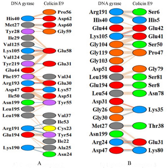
Representing the key residues by calculating the interaction between DNA Gyrase and Colicin E9 immunity protein. (A) Model #2 and (B) Model #6.
Molecular dynamics simulation
One essential technique that greatly advances the understanding of PPIs and their implications for antibacterial efficacy is MD simulation. Additionally, it facilitates exploration of mechanistic insights into the stability and binding affinities of protein-protein complexes. Additionally, MD simulations provide a comprehensive understanding of protein structure and function, which can inform the development of effective antibacterial agents. A detailed atomic-level analysis can uncover potential binding sites and mechanisms for groundbreaking antibacterial agents. This approach is especially crucial given the rise of antibiotic resistance, as it encourages the formulation of novel strategies to combat resistant bacterial strains. To explore the dynamic stability of DNA gyrase and Colicin E9 immunity protein complexes obtained from both ClusPro and LightDock tools, a long-range 300 ns MD simulation was conducted. Several statistical parameters from the MD simulation trajectories were calculated, and these are presented in Fig. 8.
Protein backbone RMSD
The protein backbone RMSD plot in Fig. 8A provides a comparative assessment of the structural integrity of the complexes formed between DNA Gyrase and the Colicin E9 immunity protein during a 300 ns MD simulation. RMSD quantifies the positional displacement of backbone atoms over time, thereby indicating structural deviations and equilibration processes in the complexes. The RMSD of DNA Gyrase (Model #2) remains comparatively low and stable during the entirety of the simulation, oscillating between 0.1 and 0.2 nm. In contrast, the RMSD of the Colicin E9 immunity protein (Model #2) exhibited greater fluctuations, attaining approximately 0.35 nm during the initial phases of simulation, particularly between 25 and 55 ns. This observation suggests that the Colicin E9 immunity protein underwent flexibility and conformational alterations before achieving a stable state. Following the initial equilibration, the RMSD stabilises at approximately 0.2 nm, and the protein interface adjusts to form a stable complex. The RMSD of DNA gyrase in Model #2 stays low and consistent throughout the simulation, fluctuating around 0.2 nm. This indicates that DNA gyrase may undergo slight conformational changes upon interaction with the Colicin E9 immunity protein in Model #6. In Model #6, the RMSD of the Colicin E9 immunity protein varies around 0.2 ns during the first 200 nanoseconds. After this initial phase, the deviations become somewhat larger than those in the Model #2 complex, suggesting that the Colicin E9 immunity protein exhibits some flexibility and undergoes conformational adjustments before stabilizing. Both complexes show stable RMSD profiles concerning DNA gyrase. Importantly, the Model #2 complex exhibits a more rigid and stable interaction, while the Model #6 complex permits greater conformational flexibility.
RMSF
The RMSF analysis provides a residue-specific assessment of the dynamic flexibility of protein complexes over the 300 ns MD simulation. RMSF quantifies the average atomic displacement of individual residues relative to their mean positions, thereby improving the identification of regions characterised by flexibility and stable binding interfaces. The amino acid residues of DNA gyrase show relatively low RMSF values in key regions, particularly in Models #2 and #6. This highlights the inherent stability of DNA gyrase during the MD simulation. In contrast, the RMSF for the Colicin E9 immunity protein in Model #6 exceeds 0.7 nm, spanning roughly 60 to 70 residues. It is crucial to emphasise that the maxima for residues 30 to 60 are notably more prominent, particularly within the context of Model #6, in which the RMSF values exceed 0.6 ns. These specific regions correspond to flexible loops and surface-exposed residues that are anticipated to undergo conformational changes during binding. The RMSF analysis reveals that DNA gyrase preserves a consistent structural conformation across both complexes, whereas the Colicin E9 immunity protein exhibits considerable flexibility, thereby enabling dynamic modulation at the binding interface. The pronounced fluctuations observed in Model #6 suggest that this framework encompasses a broader range of conformational sampling, whereas Model #2 exhibits a more rigid, compact binding configuration.
Fig. 8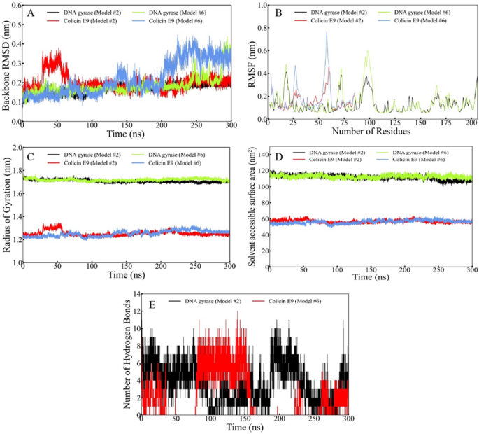
Comprehensive MD simulation analysis of the ClusPro and LightDock complexes over 300 ns. (A) Protein Backbone RMSD, (B) RMSF, (C) Radius of Gyration, (D) Solvent Accessible Surface Area, and (E) Interprotein hydrogen bonds.
RoG
The RoG analysis quantitatively evaluates the compactness and structural integrity of protein complexes throughout the 300-ns MD simulation, as shown in Fig. 8C. The RoG parameters for DNA gyrase indicate significant stability, with a consistent value of approximately 1.75 nm across the complexes, as indicated by Models #2 and #6. This consistency indicates that DNA gyrase maintains its compact, folded conformation throughout the simulation, with no observable unfolding or conformational changes. The enduring stability of the RoG for DNA gyrase highlights its structural integrity and the minimal impact of interactions with the Colicin E9 immunity protein. On the other hand, the RoG values associated with the Colicin E9 immunity protein demonstrate significant variability, highlighting its intrinsic adaptability. Regarding the Model #2 complex, the RoG attains a stable configuration at approximately 1.25 nm following an initial period characterised by minor oscillations. Conversely, the Model #6 complex shows a modest increase in fluctuations during the preliminary stages of the simulation, especially in the initial 50 ns, indicating that the flexible docking technique enables examination of a wider range of initial conformations. Finally, the RoG converges to approximately 1.25 nm over time, indicating that the Colicin E9 immunity protein adopts a compact, stable structural conformation.
SASA
The solvent exposure analysis and DNA gyrase stability in conjunction with the Colicin E9 immunity protein (Chain B/C) during the 300 ns MD simulation were performed using the SASA parameter, as shown in Fig. 8D. For DNA gyrase, the SASA analysis indicates a stable value of approximately 120 nm² for both Model #2 and Model #6 complexes. This stability indicates that DNA gyrase maintains its compact, stable structure throughout the simulation, with only slight variations in the solvent-exposed regions. These results imply that the interaction with the Colicin E9 immunity protein has minimal effect on DNA gyrase’s overall conformation or stability. In contrast, the Colicin E9 immunity protein (Model #2) exhibits greater fluctuations in SASA than DNA gyrase, highlighting its dynamic nature. Within the Model #2 complex, the SASA stabilises around 60 nm², with only minimal variability. On the other hand, the Model #6 complex shows slightly reduced fluctuations during the initial phase of the simulation, particularly within the first 50 ns, before stabilising at a comparable value of 60 nm².
Hydrogen bond analysis
The hydrogen-bond analysis shows the interaction stability between DNA gyrase and the Colicin E9 immunity protein during the 300 ns MD simulation, as shown in Fig. 8E. In the Model #2 complex, the number of hydrogen bonds remains relatively stable, fluctuating between 6 and 10 bonds for most of the frames, with occasional peaks exceeding 10 bonds. The consistency of hydrogen bonds creates a strong, well-defined interaction interface, with only slight temporal variation. In contrast, the Model #6 complex shows greater variability in the number of hydrogen bonds, ranging from 3 to 10, and we can even notice occasional spikes during specific timeframes, such as around 90–150 ns. These fluctuations suggest that the Model #6 complex undergoes conformational adjustments at the binding interface, allowing for transient interactions and optimising the interaction over time. The Model #2 complex exhibits a more consistent and rigid hydrogen-bond network, reflecting a stable binding configuration that is less susceptible to dynamic fluctuations. Both complexes exhibit interesting peaks in hydrogen-bond counts. However, the peaks in the Model #2 complex are more pronounced, indicating a strong and stable binding interface. On the other hand, the Model #6 complex supports more dynamic interactions, which are useful for modelling various physiological scenarios.
Binding free energy analysis using the MM-GBSA approach and its limitations
The MM-GBSA evaluation (Table 6) determines the binding free energy for the protein-protein complexes, breaking it down into contributions from Electrostatic Energy (EEL), Van der Waals energy, and the total binding free energy (Δtotal). The results highlight notable differences in the interactions exhibited by Models #2 and #6. The Model #2 complex shows a binding free energy of -3.88 kcal/mol, which is a much better result compared to the binding free energy of -1.62 kcal/mol seen in the Model #6 complex. This improved binding energy for Model #2 mainly comes from its strong electrostatic contributions, adding up to 531.01 kcal/mol, along with a significant boost in Van der Waals interactions, measured at -10.70 kcal/mol. These elements suggest tighter packing and improved charge stabilisation at the interface of interaction. In the Model #6 complex, despite its less favourable binding energy of -1.62 kcal/mol, it still shows steady interactions. The electrostatic energy for Model #2 is 473.80 kcal/mol, playing a crucial role in stabilising binding, although it is slightly less effective than in the ClusPro complex. In Model #6, we see that the Van der Waals energy of -6.03 kcal/mol indicates a significant degree of stabilisation from hydrophobic and dispersion forces. Additionally, the standard deviations for both complexes indicate that our energy assessments are quite reliable, with Model #2 showing slightly greater variability in its electrostatic interactions (SD = 261.56 kcal/mol). This may be due to its more rigid docking approach.
While MM-GBSA data provide a rapid assessment of the driving forces behind the Im9–DNAgyrase interaction, several caveats must be considered in the presented outcomes. Firstly, the reported values represent the effective binding enthalpy. However, to bind two proteins of interest, they must lose significant translational and rotational freedom (entropy loss), which herein does not include the solute configurational entropy, which typically imposes a significant penalty in Im9–DNA gyrase PPI associations. Secondly, the Generalized Born (GB) implicit-solvent model used in the present study might not fully capture the role of structural waters at the interface. Consequently, these values should be interpreted as a qualitative ranking of potential binding modes rather than as an absolute experimental free-energy estimate. Certainly, employing MM-GBSA in the present study neglects the significant configurational entropy loss inherent in PPI complex association; these results likely represent transient encounter states characteristic of the initial recognition phase between the non-cognate protein components and their bacterial targets.
Table 6 Binding energy of Colicin E9 immunity protein towards DNA gyrase using the MM-GBSA approach.Per residue decomposition energy
The energetic contributions of the active-site amino acid residues were explored using per-residue decomposition energy calculations. The total decomposition energy, along with its components, such as van der Waals and electrostatic energies, for the DNA gyrase active-site amino acid residues, is shown in Fig. 9. It was found that for Model #2 (Fig. 9A), except for one (ASP47), all the binding site amino acid residues, such as MET27, TYR28, ILE50, LEU54, LYS190, ARG191, ARG193, GLU194, LEU195, PHE197, LEU198, ASN199, TYR219, showed negative decomposition energy, which indicates that Colicin Im9 protein favorably exhibits binding affinity towards DNA gyrase through hydrogen bonds or van der Waals interactions. For Model #6 (Fig. 9B), ARG24, GLY26, MET27, GLY30, ASP31, ASP51, LEU54, and LEU198 showed negative per-residue binding energy, while ASP47, GLY104, ARG191, ASN199, and GLU194 exhibited positive decomposition energy. It is important to note that although a few residues had positive decomposition energy, their values were close to zero. Therefore, it is clear that Colicin Im9 showed significant affinity towards DNA gyrase in Model #6.
Fig. 9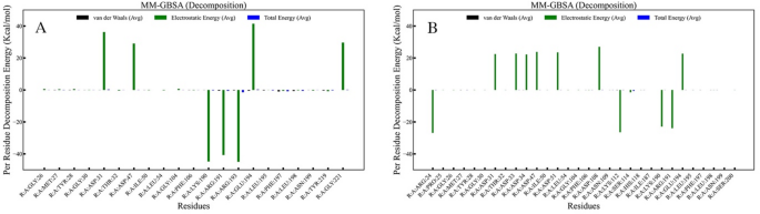
Per residue decomposition energy of the DNA gyrase binding site residues.
Principal component analysis (PCA)
The PCA plot provides a comparative depiction of the conformational landscapes investigated during the MD simulations of the protein-protein complexes generated by ClusPro and LightDock. PCA effectively distils the intricate multidimensional atomic motions into principal components, thereby furnishing a more robust representation of structural variability and stability by encapsulating the predominant modes of motion throughout the simulation.
In Model No. 2 (Fig. 10A), the PCA plot reveals a broader and more dispersed array of conformations, indicating increased structural variability and a more comprehensive sampling of conformational space throughout the simulation. This extensive distribution indicates that the interaction interface investigated a diverse range of structural states, thereby reflecting more dynamic behaviour relative to the initial rigid-body docking methodology utilised in Model #2. The observed flexibility may be attributed to structural changes that occurred during the MD simulation.
The Model #6 complex illustrated in Fig. 10B exhibits a more compact and systematically structured conformation, indicating that structural variations were successfully minimised during the simulation. In a later stage of the MD simulation, it was observed that the contact interface became well stabilised, with only slight structural changes, as evidenced by denser aggregation. This observation unites nicely with Model #6’s flexible docking method, which enabled initial adjustments that led to a highly stable binding configuration. The differences observed between the two plots illustrate the relationship between structural flexibility and stability. The expansive distribution seen in Model #2 reflects enhanced conformational exploration, whereas the tighter clustering in Model #6 suggests improved stability and a convergence toward a favoured binding state. These outcomes emphasise the complementary features of the two docking techniques, with Model #2 illustrating a more dynamic interaction framework and Model #6 highlighting structural stabilisation within protein-protein interactions.
Fig. 10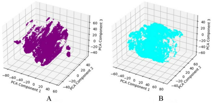
PCA plot showing the conformational space explored during MD simulations for (A) Model #2 and (B) Model #6.
Overall, the PCA plots reveal distinct conformational behaviors in the two protein-protein complexes during 300-ns MD simulations, directly correlating with their binding stabilities. In Model #2, the broader and more dispersed PCA distribution indicates greater structural variability and extensive sampling of conformational space, reflecting a more dynamic interaction interface with increased flexibility. In contrast, Model #6 showed a more compact, systematically clustered PCA plot, indicating minimized structural variations, successful convergence toward a favored binding state, and improved overall stabilization at the interface after initial adjustments. This tighter clustering in Model #6, with a stabilizing energy of -65.23 kcal/mol, aligns with its superior long-term binding stability compared to the more flexible Model #2, despite Model #2’s slightly better MM-GBSA binding free energy. These PCA patterns thus complement energetic analyses by illustrating how conformational exploration influences complex rigidity and persistence.


