


Patient and Public Involvement Statement: No patients or members of the public were involved in the design, conduct, or reporting of this trial. This decision was based on the technical nature of the machine learning framework development and the use of retrospective anonymized fitness assessment data.
Data collection and preprocessingModel development cohort (retrospective dataset)
The data for developing and training the machine learning model came from a retrospective, anonymized database of 6,698 male undergraduate students (hereafter referred to as the model-development cohort) recruited from Changsha Aeronautical Vocational and Technical College, Hunan province, China, selected through a stratified random sampling strategy to ensure representative demographic and geographic distribution. Participants exhibited homogeneous age distribution (mean = 18.7 ± 0.9 years; range: 18–20 years), consistent with the standardized age distribution of first-year university students in China. Body Mass Index (BMI) was classified according to World Health Organization (WHO) guidelines, revealing the following distribution: underweight (BMI < 18.5 kg/m2), 5.3%; normal weight (18.5–24.9 kg/m2), 74.5%; overweight (25–29.9 kg/m2), 19.0%; and obese (≥ 30 kg/m2), 1.2%. This skewed distribution aligns with national epidemiological trends showing rising overweight prevalence among urban youth. Exclusion criteria comprised self-reported chronic diseases, recent musculoskeletal injuries, and participation in competitive sports programs, ensuring a focus on general population health.
Sample size justification: The target sample size was calculated to detect a clinically meaningful BMI reduction of ≥ 1.5 kg/m2 (SD = 2.0) between groups, with 90% power at α = 0.05 (two-tailed). Accounting for 15% attrition, the required sample was 580 per group. The final cohort (n = 6,698) exceeded this threshold to ensure robust subgroup analyses and representativeness.
Intervention trial cohort (prospective RCT)
To empirically validate the prescription framework, a separate, prospective 12-week randomized controlled trial (RCT) was conducted. A new cohort of participants (hereafter referred to as the intervention cohort) was recruited from the same institution, distinct from the development dataset. The sample size calculation and randomization procedures are described in Sect. 2.4. After accounting for an estimated 15% attrition, a total of 1,160 participants (580 per group) were required and successfully enrolled for the intervention study.
Fitness test battery
A comprehensive fitness assessment protocol was employed to quantify four critical physiological domains: aerobic capacity, muscular strength, core endurance, and anaerobic power. All testing procedures strictly adhered to standardized protocols validated by the Chinese National Student Physical Fitness Standard:
1)
3,000-meter run: Aerobic endurance was assessed using a radio-frequency identification (RFID) timing system (Zebra Technologies, USA), with 200-meter interval splits captured to evaluate pacing dynamics and fatigue development. Participants completed the test on a synthetic track under controlled environmental conditions (ambient temperature: 22–25 °C; relative humidity: 50–60%).
2)
Pull-up test: Maximal upper-body strength was quantified by counting the highest number of consecutive pull-up test performed with standardized form (full elbow extension at the bottom position and clear chin elevation above the bar plane at the top position). The test was terminated upon failure to complete a repetition within 5 s.
3)
Sit-up test: Core muscular endurance was assessed by the maximum number of properly performed sit-up test (with hands maintained in a crossed position over the chest, full trunk flexion until both elbows contacted the thighs) completed within 60 s. A lumbar support pad was used to ensure spinal safety.
4)
30 × 2 shuttle run: Anaerobic power output was quantified by the total time taken to complete 30 shuttle sprints over a 4-meter distance, measured using infrared timing gates (Brower Timing Systems, USA) with an accuracy of ± 0.01 s.
All tests were conducted by certified trainers, demonstrating excellent intra-rater reliability (Cohen’s κ > 0.92) across repeated measurements.
Data augmentation
To mitigate the severe class imbalance in BMI categories (especially the 1.2% obesity prevalence), a two-stage data augmentation strategy was developed:
1)
Synthetic Minority Oversampling Technique (SMOTE): The SMOTE generated synthetic samples for underrepresented classes (underweight, overweight, obese) by interpolating between nearest neighbors (k = 5) in the feature space. This process balanced class distributions by augmenting minority samples to match the majority class (normal weight), while preserving original data variance structure.
2)
Gaussian Noise Injection: To improve model robustness against measurement variability, zero-mean Gaussian noise (σ = 0.1) was applied to both synthetic and original samples. This regularization technique enhanced generalization performance by emulating real-world data noise and artifacts, including minor timing discrepancies or physiological fluctuations.
Following data augmentation, the training dataset expanded to 19,944 samples (4,986 per BMI category), ensuring balanced class representation for classifier training. To prevent data leakage and over-optimistic performance estimation, all data augmentation techniques (SMOTE and Gaussian noise injection) were applied only within the training folds of the stratified 5-fold cross-validation loop. The validation and test folds in each iteration contained only original, non-synthetic data. The augmentation efficacy was rigorously validated via stratified 5-fold cross-validation, demonstrating a 12.4% improvement in classification accuracy compared with the non-augmented baseline.
Hybrid model architecture
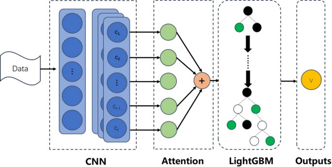
This study proposes a hybrid machine learning framework that integrates deep learning with gradient boosting techniques to achieve high-accuracy BMI classification and personalized exercise prescription generation through multidimensional fitness data. The framework comprises three core modules: a feature extractor based on 1D-CNN and multi-head attention, a LightGBM classifier, and an interpretability-driven exercise prescription algorithm. This section details the design rationale and implementation of each module.
Feature extraction branch
This module integrated 1D-CNN with multi-head attention to extract both local temporal patterns and global contextual features from sequential fitness data (e.g., 3,000-meter run lap times). The detailed structure is as follows:
1)
Input layer: Accepts sequential data with shape X∈RN×T×F, where N is the number of samples, T = 15 represents the 15 consecutive 200-meter lap time intervals extracted from the 3,000-meter run, and F = 4 corresponds to the four fitness metrics. To form a consistent multivariate time-series input for the 1D-CNN, the single-measurement values for the other three tests—pull-up count (repetitions), sit-up count (repetitions in 60s), and total 30 × 2 shuttle run time (seconds)—are replicated across all T = 15 time steps for each participant. This structure allows the convolutional kernels to capture localized temporal patterns in running pace while being concurrently informed by the replicated values of strength, endurance, and anaerobic power metrics. For example, a participant’s input matrix would have lap times varying across rows 1–15, while each row also contains the same three constant values for that participant’s pull-up test, sit-up test, and 30 × 2 shuttle run time.
2)
The 1D convolutional block: It consists of three convolutional layers with filter sizes of 64, 128, and 256, respectively. Each layer employs a kernel size of 5, stride of 2, and ReLU activation function. Through strided convolution, the network progressively reduces the sequence length (T→⌈ T/2⌉ →⌈ T/4⌉ →⌈ T/8⌉ ) while simultaneously increasing feature depth. The operation at the l-th layer is defined as:
$${{\text{H}}^{\left( l \right)}}={\text{ReLU}}({{\text{W}}^{\left( l \right)}}*{{\text{H}}^{(l\, – \,1)}}\,+\,{{\text{b}}^{\left( l \right)}}),$$
where \({{\text{W}}^{(l)}} \in {{\text{R}}^{k \times {d_{in}} \times {d_{out}}}}\) denotes the convolutional kernel (kernel length k = 5, input/output channels din, dout), and the stride is s = 2.
3)
Multi-head attention: The attention mechanism consists of eight parallel attention heads, with each head using 32-dimensional projections for the query, key, and value vectors. Scaled dot-product attention is computed for each head, followed by dropout with a rate of 0.3 to enhance regularization. The resulting outputs are aggregated with CNN features via residual connections. Let HCNN∈RN×T′×d denote the CNN output features from the CNN. These features undergo linear projections to generate the queries (Q), keys (K), and values (V), each with dimensions RN×h×T′×d/h, where h = 8 represents the number of attention heads. The scaled dot-product attention is computed as:
$${\text{Attention}}(Q,K,V)={\text{soft}}\,{\text{max}}\left( {\frac{{Q{K^T}}}{{\sqrt {d/h} }}} \right)V.$$
The outputs from all attention heads are concatenated and integrated via residual connections and layer normalization:
$${{\text{H}}_{{\text{attn}}}}={\text{LayerNorm }}({{\text{H}}_{{\text{CNN}}}}+{\text{Concat}}({\text{hea}}{{\text{d}}_{\text{1}}}, \ldots ,{\text{ hea}}{{\text{d}}_h}){{\text{W}}^O}),$$
where WO∈Rd×d is the output projection matrix.
4)
Feature pooling: A global average pooling operation is applied to produce a 256-dimensional fixed-length feature vector z∈Rd:
$$z=\frac{1}{{{T^{\prime}}}}\sum\limits_{{t=1}}^{{T^{\prime}}} {{{\text{H}}_{{\text{attn}}}}[:,t,:]}$$
LightGBM classifier
The feature vector z extracted from the 1D-CNN + Attention module was fed into a LightGBM classifier. The objective function incorporated a regularized logistic loss:
$${L_{GBM}}=\sum\limits_{{i=1}}^{N} {[{y_i}\log {p_i}+(1 – {y_i})\log (1 – {p_i})]+{\lambda _1}{{\left\| \theta \right\|}_1}+{\lambda _2}\left\| \theta \right\|_{2}^{2}} ,$$
where \({p_i}=\sigma \left( {\sum\limits_{{m=1}}^{M} {{f_m}({z_i})} } \right)\), fm denotes the prediction from the m-th tree, \({\lambda _1}=1.2\), and \({\lambda _2}=0.8\).
Custom loss function
The total loss integrates weighted fitness metric losses with an attention regularization term:
$${L_{{\text{total}}}}=0.{\text{4}}{L_{{\text{3}}000{\text{m}}}}+0.{\text{2}}{L_{{\text{Pull}} – {\text{Ups}}}}+0.{\text{2}}{L_{{\text{Sit}} – {\text{Ups}}}}+0.{\text{2}}{L_{{\text{Shuttle}}}}+\lambda {L_{{\text{Attention}}}}.$$
The weights were assigned based on feature importance analysis, with an attention regularization term (λ = 0.1) employed to enforce sparsity in the attention weights.
Model training and optimization
1) Training Strategy:
The 1D-CNN + Attention feature extractor was optimized using the Adam optimizer with a learning rate (lr) of 0.001, a first-moment decay rate (β1) of 0.9, and a second-moment decay rate (β2) of 0.999. The custom loss function (Sect. 3.2.3) was used during this stage.To mitigate class imbalance and evaluate model generalizability, a stratified 5-fold cross-validation scheme was applied to the training folds of the augmented dataset (N = 19,944 samples after augmentation, applied only to training data). The stratification ensured that each fold maintained proportional representation of BMI categories. After training the feature extractor, the fixed-length feature vector z was extracted for all samples. A LightGBM classifier was then trained separately on these extracted features using its native gradient boosting algorithm and the same 5-fold cross-validation scheme, ensuring no overlap between training and evaluation data across stages. Performance metrics were averaged across all folds to minimize sampling bias.
Training was terminated if the validation loss showed no improvement for 10 consecutive epochs. This early stopping criterion prevented overfitting by halting optimization before the model began memorizing noise introduced by synthetic samples. The patience threshold (patience = 10) was empirically validated through preliminary tests to, balance computational resource constraints with convergence stability.
2) Regularization:
An L2 regularization term (λ = 10− 4) was applied to all trainable parameters, including convolutional filters and attention projection matrices. This penalty term effectively suppresses excessive weight growth, constrains model complexity and reduces the risk of overfitting to minority classes. The λ value was optimized through grid search on a held-out validation subset to achieve an optimal bias-variance tradeoff.
To simulate real-world measurement variability and enhance robustness, Gaussian noise (σ = 0.05) was injected into feature interactions during training. Specifically, the noise was introduced at the concatenated outputs of the 1D-CNN and multi-head attention layers prior to the pooling operation. This technique disrupted spurious correlations between localized temporal patterns and BMI labels, thereby promoting the learning of invariant feature representations. The noise magnitude (σ) was calibrated to avoid masking meaningful signal variance. Ablation studies demonstrated a 7.3% improvement in cross-validation F1 scores compared with noise-free training.
3) Integration with Prescription Algorithm:
The optimized model outputs are dynamically linked to the exercise prescription algorithm via SHAP-derived feature importance scores. For instance, the attention weights that emphasize fatigue patterns in the final laps of 3,000-meter runs are utilized to precisely tailor aerobic training volume, ensuring alignment with individual physiological responses. This closed-loop integration between model training and intervention adaptation highlights the framework’s dynamic evolution capability alongside participant progress, representing a significant advancement beyond static exercise guidelines.
This study proposes a computational framework for personalized health behavior intervention, integrating adaptive optimization techniques with strict regularization protocols. The core operational mechanism of this framework comprises four main modules: data acquisition and preprocessing, feature extraction, model training and optimization, and personalized guidance and feedback.
The framework achieved state-of-the-art performance (94.5% accuracy) while maintaining real-time inference efficiency (< 0.8 ms/sample) (see Fig. 1).
Fig. 1 The alternative text for this image may have been generated using AI.Prescription algorithmData processing and initial prescription formulation
Participants in the intervention cohort underwent comprehensive physical fitness assessments consisting of four standardized tests drawn from internationally validated protocols in sports science and clinical practice: the 3,000-meter run, the pull-up test, the sit-up test, and the 30 × 2 shuttle run. Specifically, these tests evaluate key dimensions of physical performance, namely, aerobic capacity (3,000-meter run), muscular strength (pull-up test), muscular endurance (sit-up test), and anaerobic capacity (30 × 2 shuttle run). They were selected as core evaluation metrics for this study because they effectively reflect participants’ physical fitness levels and demonstrate strong associations with health conditions such as overweight and obesity.
The collected data underwent preprocessing procedures, including feature normalization, to ensure dimensional consistency and optimize AI analysis. Using the preprocessed data, an initial exercise prescription was formulated by the AI model. These processed data were subsequently utilized by the AI model to generate preliminary exercise prescriptions. This was achieved through a rule-based algorithm that translated the AI model’s output into actionable prescriptions. The process involved three sequential steps:
(1) Model Inference & Interpretation
For each participant, the trained hybrid model provided a BMI class prediction and the associated SHAP (SHapley Additive exPlanations) values for the four input fitness features.
(2) Deficiency Prioritization
Features were ranked by their mean absolute SHAP value within the individual’s prediction. The top 1–2 features with the highest positive SHAP contributions (indicating a strong association with a less healthy BMI category) were identified as the primary fitness deficiencies to target.
(3) Prescription Mapping
Based on pre-defined, evidence-based mapping rules, the prioritized deficiencies were linked to specific exercise modalities.
For instance, a high positive SHAP value for pull-up count (indicating low strength contributed to a higher BMI prediction) triggered a focus on upper-body resistance training in the weekly regimen. Similarly, a high positive SHAP value for 3,000-meter run time triggered an emphasis on aerobic conditioning. The generic training protocols (e.g., HIIT, Aerobic Exercise, Strength Training outlined in Table 1) served as templates, and their relative weekly volume and emphasis were adjusted according to this deficiency-priority mapping.
Data reassessment and prescription adjustment
To validate the effectiveness and rationality of the proposed exercise prescription, a 12-week intervention trial was conducted involving the intervention cohort (N = 1160). Participants were randomly and equally assigned to either the intervention group (receiving personalized exercise prescriptions) or the control group (following routine exercise protocols). The study design was rigorously controlled to minimize measurement errors and external confounding variables, as detailed in Table 1.
Table 1 Personalized exercise intervention protocol.
Requirements:
1)
Baseline Data Assessment and Initial Prescription Deployment: At the beginning of the intervention, baseline fitness test results were recorded and input into the AI model to determine individual baseline performance levels. Based on these assessments, initial exercise prescriptions were formulated and tailored to address specific fitness deficiencies.
2)
Iterative Data Collection and Performance Evaluation: Throughout the intervention period, data were collected at regular intervals (e.g., biweekly) to monitor progress. The AI model reassessed these data, comparing them with both baseline measurements and prior assessments to evaluate the effectiveness of the current prescription.
3)
Prescription Adjustment: For domains showing improvement, the prescription either remained unchanged or was slightly modified to maintain progress. For domains exhibiting stagnation or decline, the AI model intensified the prescription by increasing training volume, frequency, or intensity. Additionally, the AI model monitored the fatigue-recovery balance index (FRBI) to detect signs of overtraining. Participants with FRBI > 1.2 automatically experienced a 15–20% reduction in load for 3–5 days to promote recovery.
Continuous reassessment and optimization
The process of data reassessment and prescription adjustment was continuous, ensuring that the exercise prescription remained optimized throughout the intervention period. At the conclusion of the intervention, a final reassessment was conducted to evaluate the overall effectiveness of the personalized exercise prescription. Based on these results, the AI model was fine-tuned to enhance future interventions.
Randomization and blinding
Randomization:
An independent statistician generated allocation sequences using permuted block design (block size = 4) via SAS PROC PLAN. Sequentially numbered opaque envelopes secured allocation concealment.
Blinding:
Outcome assessors (fitness testers) were blinded to group assignment. Participants and trainers were unblinded due to intervention nature.